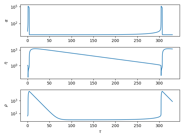
常微分方程式の数値解法(6)
SciPyのodeintを用いて以下のOrdinary Differential Equations (ODE)を解き,文献[1]の数値解を再現する.
ここで,,
,
,
であり,初期値は
,
,
とした.
[1] Field, R. J. and Noyes, R. M., Oscillations in chemical systems. IV. Limit cycle behavior in a model of a real chemical reaction, J. Chem. Phys., 60(5), 1877-1884 (1974)
#
# Field, R. J. and Noyes, R. M.,
# Oscillations in chemical systems. IV.
# Limit cycle behavior in a model of a real chemical reaction,
# J. Chem. Phys., 60(5), 1877-1884 (1974)
#
import numpy as np
from scipy.integrate import odeint
import matplotlib.pyplot as plt

# right-hand side
def rhs(y, x, s, q, f, w):
    return [s*(y[1] - y[1]*y[0] + y[0] - q*y[0]**2),
            (- y[1] - y[0]*y[1] + f*y[2])/s,
            w*(y[0] - y[2])]

# parameters
s = 77.27
q = 8.375e-6
f = 1.0
w = 0.1610

# initial condition
y0 = [4.0, 1.1, 4.0]

# output interval
x = np.arange(0.0, 330.0, 0.1)

# solve ode
y = odeint(rhs, y0, x, args=(s, q, f, w))

# output
figs = plt.figure()
fig1 = figs.add_subplot(3, 1, 1)
fig2 = figs.add_subplot(3, 1, 2)
fig3 = figs.add_subplot(3, 1, 3)
fig1.set_yscale('log')
fig1.set_ylabel(r'$\alpha$')
fig1.plot(x, y[:,0])
fig2.set_yscale('log')
fig2.set_ylabel(r'$\eta$')
fig2.plot(x, y[:,1])
fig3.set_yscale('log')
fig3.set_xlabel(r'$\tau$')
fig3.set_ylabel(r'$\rho$')
fig3.plot(x, y[:,2])
figs.tight_layout()
#plt.show()
plt.savefig('Field1974.png')
常微分方程式の数値解法(5)
SciPyのodeintを用いて以下のOrdinary Differential Equations (ODE)を解き,文献[1,2]のChemical Akzo Nobel problemの数値解を再現する.
[1] Amat, S. et al., On a Variational Method for Stiff Differential Equations Arising from CHemistry Kinetics, Mathematics, 7, 459 (2019) [2] Kafash, B. et al., Chemical Akzo Nobel Problem; Mathematical Description and Its Solution Via Model Maker Software, MATCH Commum. Math. Comput. Chem., 71, 279-286 (2014)

#
# Chemical Akzo Nobel Problem in
#
# [1] Amat, S. et al.,
#     On a Variational Method for Stiff Differential Equations
#     Arising from CHemistry Kinetics,
#     Mathematics, 7, 459 (2019)
#
# [2] Kafash, B. et al.,
#     Chemical Akzo Nobel Problem; Mathematical Description
#     and Its Solution Via Model Maker Software,
#     MATCH Commum. Math. Comput. Chem., 71, 279-286 (2014)
#
import numpy as np
from scipy.integrate import odeint
import matplotlib.pyplot as plt

# right-hand side
def rhs(y, x, k0, k1, k2, K, k3, klA, Ks, p, H):

    r0 = k0 * y[0]**4 * np.sqrt(y[1])
    r1 = k1 * y[2] * y[3]
    r2 = k1 * y[0] * y[4] / K
    r3 = k2 * y[0] * y[3]**2
    y5 = Ks * y[0] * y[3]
    r4 = k3 * y5**2 * np.sqrt(y[1])
    Fin = klA * (p / H - y[1])

    yp0 = - 2.0 * r0 + r1 - r2 - r3
    yp1 = - 0.5 * r0 - r3 - 0.5e0 * r4 + Fin
    yp2 = r0 - r1 + r2
    yp3 = - r1 + r2 - 2.0 * r3
    yp4 = r1 - r2 + r4
    return [yp0, yp1, yp2, yp3, yp4]

# parameters
k0 = 18.7
k1 = 0.58
k2 = 0.09
K = 34.4
k3 = 0.42
klA = 3.3
Ks = 115.83
p = 0.9
H = 737.0

# initial condition
# 0: FLB, 1: CO2, 2: FLBT, 3: ZHU, 4: ZLA, 5: FLB.ZHU
FLB     = 0.444
CO2     = 0.00123
FLBT    = 0.0
ZHU     = 0.007
ZLA     = 0.0
FLB_ZHU = 0.367
ZHU     = FLB_ZHU/(Ks*FLB)
y0      = [FLB, CO2, FLBT, ZHU, ZLA]

# output interval
x = np.arange(0.0, 200.0, 0.1)

# solve ode
y = odeint(rhs, y0, x, args = (k0, k1, k2, K, k3, klA, Ks, p, H))

# output
plt.xlabel('t')
plt.ylabel('y')
plt.plot(x, y[:,0],           label='FLB')
plt.plot(x, y[:,1]*1e2,       label='CO2 (\u00d7$10^2$)')
plt.plot(x, y[:,2],           label='FLBT')
plt.plot(x, y[:,3]*1e1,       label='ZHU (\u00d7$10^1$)')
plt.plot(x, y[:,4]*1e1,       label='ZLA (\u00d7$10^1$)')
plt.plot(x, Ks*y[:,0]*y[:,3], label='FLB.ZHU')
plt.legend()
#plt.show()
plt.savefig('ChemicalAkzoNobelProblem.png')
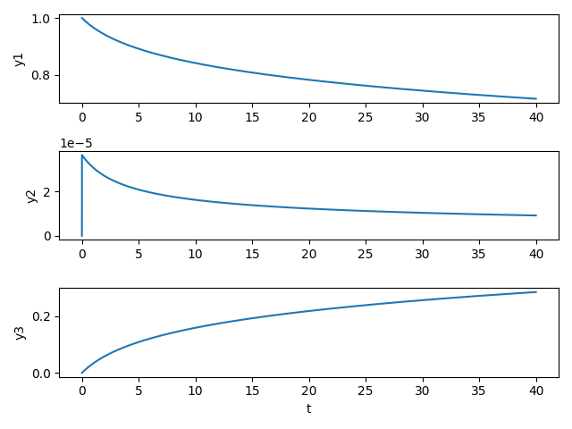
常微分方程式の数値解法(4)
SciPyのodeintを用いて以下のOrdinary Differential Equations (ODE)を解き,文献[1]のProblem HIRESの数値解を再現する.
[1] Amat, S. et al., On a Variational Method for Stiff Differential Equations Arising from Chemistry Kinetics, Mathematics, 7, 459 (2019)

#
# Problem HIRES
#
import numpy as np
from scipy.integrate import odeint
import matplotlib.pyplot as plt

# right-hand side
def rhs(y, x):
        return[- 1.71*y[0] + 0.43*y[1] + 8.32*y[2] + 0.0007,
                 1.71*y[0] - 8.75*y[1],
               - 10.03*y[2] + 0.43*y[3] + 0.035*y[4],
                 8.32*y[1] + 1.71*y[2] - 1.12*y[3],
               - 1.745*y[4] + 0.43*y[5] + 0.43*y[6],
               - 280.0*y[5]*y[7] + 0.69*y[3] + 1.71*y[4] - 0.43*y[5] + 0.69*y[6],
                 280.0*y[5]*y[7] - 1.81*y[6],
               - 280.0*y[5]*y[7] + 1.81*y[6]]

# initial condition
y0 = [1.0,0.0,0.0,0.0,0.0,0.0,0.0,0.0057]

# output interval
x = np.arange(0.0,400.0,0.01)

# solve ode
y = odeint(rhs, y0, x)

# outout
figs = plt.figure(figsize=(6.4,4.8*2))
fig1 = figs.add_subplot(4, 2, 1)
fig2 = figs.add_subplot(4, 2, 2)
fig3 = figs.add_subplot(4, 2, 3)
fig4 = figs.add_subplot(4, 2, 4)
fig5 = figs.add_subplot(4, 2, 5)
fig6 = figs.add_subplot(4, 2, 6)
fig7 = figs.add_subplot(4, 2, 7)
fig8 = figs.add_subplot(4, 2, 8)
fig1.set_xlim(0.0,5.0)
fig2.set_xlim(0.0,5.0)
fig3.set_xlim(0.0,5.0)
fig4.set_xlim(0.0,5.0)
fig5.set_xlim(0.0,400.0)
fig6.set_xlim(0.0,400.0)
fig7.set_xlim(0.0,5.0)
fig8.set_xlim(0.0,5.0)
fig1.set_ylabel('y1')
fig2.set_ylabel('y2')
fig3.set_ylabel('y3')
fig4.set_ylabel('y5')
fig5.set_ylabel('y5')
fig6.set_ylabel('y6')
fig7.set_ylabel('y7')
fig8.set_ylabel('y8')
fig7.set_xlabel('t')
fig8.set_xlabel('t')
fig1.plot(x, y[:,0])
fig2.plot(x, y[:,1])
fig3.plot(x, y[:,2])
fig4.plot(x, y[:,3])
fig5.plot(x, y[:,4])
fig6.plot(x, y[:,5])
fig7.plot(x, y[:,6])
fig8.plot(x, y[:,7])
figs.tight_layout()
#plt.show()
figs.savefig('tmp.png')
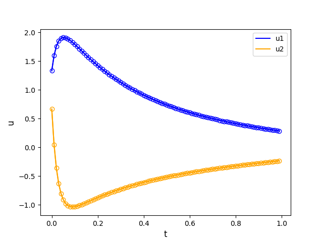
常微分方程式の数値解法(3)
SciPyのodeintを用いて以下の厳密解のあるOrdinary Differential Equations (ODE)を解き,文献[1]の数値解を再現する.
なお,文献[1]のの右辺第3項の
は
の間違いである.これら常微分方程式の厳密解は以下に示すとおりである.
[1] Thohura, S. and Rahman, A., Numerical Approach for Solving Stiff Differential Equations: A Comparative Study, GLOBAL JOURNAl OF SCIENCE FRONTIER RESEARCH MATHEMATICS AND DECISION SCIENCES, 13 (6) (2013)
#
# Thohura, S. and Rahman, A.,
# Numerical Approach for Solving Stiff Differential Equations:
# A Comparative Study,
# GLOBAL JOURNAl OF SCIENCE FRONTIER RESEARCH
# MATHEMATICS AND DECISION SCIENCES, 13 (6) (2013)
#
import numpy as np
from scipy.integrate import odeint
import matplotlib.pyplot as plt

# right-hand side
def rhs(y, x):
    return [ 9.0*y[0] + 24.0*y[1] + 5.0*np.cos(x) - np.sin(x)/3.0,
           -24.0*y[0] - 51.0*y[1] - 9.0*np.cos(x) + np.sin(x)/3.0]

# exact solution
def exact(x):
    return [2.0*np.exp(-3.0*x) -     np.exp(-39.0*x) + np.cos(x)/3.0,
           -    np.exp(-3.0*x) + 2.0*np.exp(-39.0*x) - np.cos(x)/3.0]

# initial condition
y0 = [4.0/3.0, 2.0/3.0]

# output interval
x = np.arange(0.0, 1.0, 0.01)

# solve ode
y = odeint(rhs, y0, x)

#y_e = [[0 for i in range(100)] for j in range(2)]
y_e = np.empty((100, 2))

# exact solution
i = 0
for t in x:
    y_e[i,:] = exact(t)
    i += 1

# output
plt.xlabel('t')
plt.ylabel('u')
plt.plot(x, y_e[:,0],marker='o', markerfacecolor='none',color='blue')
plt.plot(x, y_e[:,1],marker='o', markerfacecolor='none',color='orange')
plt.plot(x, y[:,0], label='u1', color='blue')
plt.plot(x, y[:,1], label='u2', color='orange')
plt.legend()
#plt.show()
plt.savefig('Thohura2013-Fig2.png')
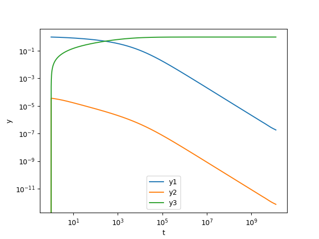
常微分方程式の数値解法(2)
SciPyのodeintを用いて以下のOrdinary Differential Equations (ODE)を解き,文献[1,2]のRobertson problemの数値解を再現する.
ここで,初期値,
,
である.
[1] Thohura, S. and Rahman, A., Numerical Approach for Solving Stiff Differential Equations: A Comparative Study, GLOBAL JOURNAl OF SCIENCE FRONTIER RESEARCH MATHEMATICS AND DECISION SCIENCES, 13 (6) (2013)
[2] The Robertson Problem — Dymos
#
# Robertson problem in
# Thohura, S. and Rahman, A.,
# Numerical Approach for Solving Stiff Differential Equations:
# A Comparative Study,
# GLOBAL JOURNAl OF SCIENCE FRONTIER RESEARCH
# MATHEMATICS AND DECISION SCIENCES, 13 (6) (2013)
#
import numpy as np
from scipy.integrate import odeint
import matplotlib.pyplot as plt

# right-hand side
def rhs(y, x):
    k1 = 0.04
    k2 = 3e7
    k3 = 1e4
    return [-k1*y[0] + k3*y[1]*y[2],
             k1*y[0] - k3*y[1]*y[2] - k2*y[1]**2,
                                      k2*y[1]**2]

# initial condition
y0 = [1.0, 0.0, 0.0]

# output interval
p = np.arange(0.0, 10.1, 0.001)
x = np.empty(10100)
i = 0
for t in p:
    x[i] = 10.0**t
    i += 1

# solve ode
y = odeint(rhs, y0, x)

# output
plt.xlabel('t')
plt.ylabel('y')
plt.xscale('log')
plt.yscale('log')
plt.plot(x, y[:,0], label='y1')
plt.plot(x, y[:,1], label='y2')
#plt.plot(x, y[:,1]*1e4)
plt.plot(x, y[:,2], label='y3')
plt.legend()
#plt.show()
plt.savefig('Thohura2013-Fig1.png')
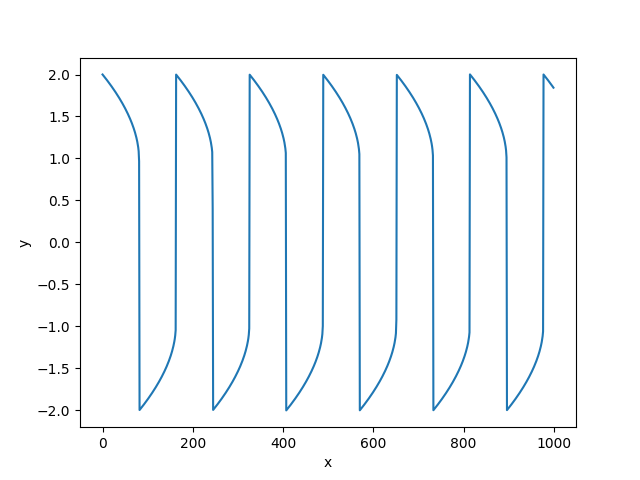
常微分方程式の数値解法(1)
SciPyのodeintを用いて以下のOrdinary Differential Equations (ODE)を解き,文献[1]の数値解を再現する.
ここで,,初期値
,
である.
[1] Petzold, L., Automatic selection of methods for solving stiff and nonstiff systems of ordinary differential equations, SIAM, J. Sci. Stat. Comput., 5(1), 136-148 (1983)
#
# Van der Pol's equation in
# Petzold, L.,
# Automatic selection of methods for solving stiff and nonstiff systems
# of ordinary differential equations,
# SIAM J. Sci. Stat. Comput., 4(1), 136-148 (1983)
#
import numpy as np
from scipy.integrate import odeint
import matplotlib.pyplot as plt

# constant
eta = 100.0

# right-hand side
def func(y, x, eta):
    return [y[1],
            eta*(1 - y[0]**2)*y[1] - y[0]]

# initial condition
y0 = [2.0, 0.0]

# output interval
x = np.arange(0.0, 1000.0, 1.0)

# solve ode
y = odeint(func, y0, x, args=(eta,))

# output
plt.xlabel('x')
plt.ylabel('y')
plt.plot(x, y[:,0])
#plt.plot(x, y[:,1])
#plt.show()
plt.savefig('Petzold1983-Fig1.png')
EnSight Goldフォーマット
以前,ParaViewを用いた可視化に用いるデータファイルのフォーマットにはEnSight Goldフォーマットが良いと述べたが,EnSight Goldのファイルフォーマットは以下のドキュメントのSection 11.1 EnSight Gold CaseFile Formatで厳格に定義されている.