常微分方程式の数値解法(6) - 流体解析のあれこれ

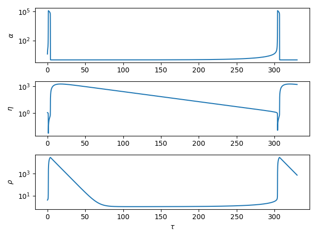
SciPyのodeintを用いて以下のOrdinary Differential Equations (ODE)を解き，文献[1]の数値解を再現する．

$\displaystyle d \alpha / d \tau = s \left( \eta - \eta \alpha + \alpha -q \alpha^2 \right)$

$\displaystyle d \eta / d \tau = s^{-1} \left( - \eta - \eta \alpha + f \rho \right)$

$\displaystyle d \rho / d \tau = w \left( \alpha - \rho \right)$

ここで， $s = 77.27$ ， $q = 8.375 \times 10^{-6}$ ， $f = 1.0$ ， $w = 0.1610$ であり，初期値は $\alpha = 4.0$ ， $\eta = 1.1$ ， $\rho = 4.0$ とした．

[1] Field, R. J. and Noyes, R. M., Oscillations in chemical systems. IV. Limit cycle behavior in a model of a real chemical reaction, J. Chem. Phys., 60(5), 1877-1884 (1974)

#
# Field, R. J. and Noyes, R. M.,
# Oscillations in chemical systems. IV.
# Limit cycle behavior in a model of a real chemical reaction,
# J. Chem. Phys., 60(5), 1877-1884 (1974)
#
import numpy as np
from scipy.integrate import odeint
import matplotlib.pyplot as plt

# right-hand side
def rhs(y, x, s, q, f, w):
    return [s*(y[1] - y[1]*y[0] + y[0] - q*y[0]**2),
            (- y[1] - y[0]*y[1] + f*y[2])/s,
            w*(y[0] - y[2])]

# parameters
s = 77.27
q = 8.375e-6
f = 1.0
w = 0.1610

# initial condition
y0 = [4.0, 1.1, 4.0]

# output interval
x = np.arange(0.0, 330.0, 0.1)

# solve ode
y = odeint(rhs, y0, x, args=(s, q, f, w))

# output
figs = plt.figure()
fig1 = figs.add_subplot(3, 1, 1)
fig2 = figs.add_subplot(3, 1, 2)
fig3 = figs.add_subplot(3, 1, 3)
fig1.set_yscale('log')
fig1.set_ylabel(r'$\alpha$')
fig1.plot(x, y[:,0])
fig2.set_yscale('log')
fig2.set_ylabel(r'$\eta$')
fig2.plot(x, y[:,1])
fig3.set_yscale('log')
fig3.set_xlabel(r'$\tau$')
fig3.set_ylabel(r'$\rho$')
fig3.plot(x, y[:,2])
figs.tight_layout()
#plt.show()
plt.savefig('Field1974.png')