常微分方程式の数値解法(3) - 流体解析のあれこれ

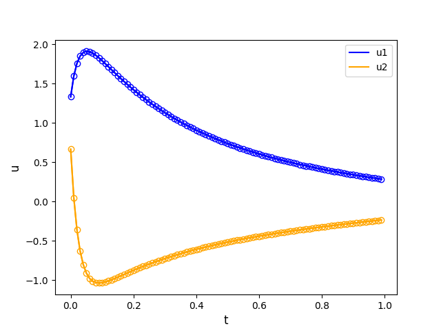
SciPyのodeintを用いて以下の厳密解のあるOrdinary Differential Equations (ODE)を解き，文献[1]の数値解を再現する．

$\displaystyle u_1^{\prime} = 9 u_1 + 24 u_2 + 5 \cos t - \dfrac{1}{3} \sin t$

$\displaystyle u_2^{\prime} = - 24 u_1 - 51 u_2 - 9 \cos t + \dfrac{1}{3} \sin t$

なお，文献[1]の $u_2^{\prime}$ の右辺第3項の $-95 \cos t$ は $-9 \cos t$ の間違いである．これら常微分方程式の厳密解は以下に示すとおりである．

$\displaystyle u_1 \left( t \right) = 2 e^{-3 t} - e^{-39 t} + \dfrac{1}{3} \cos t$

$\displaystyle u_2 \left( t \right) = - e^{-3 t} + 2 e^{-39 t} - \dfrac{1}{3} \cos t$

$\displaystyle$

[1] Thohura, S. and Rahman, A., Numerical Approach for Solving Stiff Differential Equations: A Comparative Study, GLOBAL JOURNAl OF SCIENCE FRONTIER RESEARCH MATHEMATICS AND DECISION SCIENCES, 13 (6) (2013)

#
# Thohura, S. and Rahman, A.,
# Numerical Approach for Solving Stiff Differential Equations:
# A Comparative Study,
# GLOBAL JOURNAl OF SCIENCE FRONTIER RESEARCH
# MATHEMATICS AND DECISION SCIENCES, 13 (6) (2013)
#
import numpy as np
from scipy.integrate import odeint
import matplotlib.pyplot as plt

# right-hand side
def rhs(y, x):
    return [ 9.0*y[0] + 24.0*y[1] + 5.0*np.cos(x) - np.sin(x)/3.0,
           -24.0*y[0] - 51.0*y[1] - 9.0*np.cos(x) + np.sin(x)/3.0]

# exact solution
def exact(x):
    return [2.0*np.exp(-3.0*x) -     np.exp(-39.0*x) + np.cos(x)/3.0,
           -    np.exp(-3.0*x) + 2.0*np.exp(-39.0*x) - np.cos(x)/3.0]

# initial condition
y0 = [4.0/3.0, 2.0/3.0]

# output interval
x = np.arange(0.0, 1.0, 0.01)

# solve ode
y = odeint(rhs, y0, x)

#y_e = [[0 for i in range(100)] for j in range(2)]
y_e = np.empty((100, 2))

# exact solution
i = 0
for t in x:
    y_e[i,:] = exact(t)
    i += 1

# output
plt.xlabel('t')
plt.ylabel('u')
plt.plot(x, y_e[:,0],marker='o', markerfacecolor='none',color='blue')
plt.plot(x, y_e[:,1],marker='o', markerfacecolor='none',color='orange')
plt.plot(x, y[:,0], label='u1', color='blue')
plt.plot(x, y[:,1], label='u2', color='orange')
plt.legend()
#plt.show()
plt.savefig('Thohura2013-Fig2.png')