常微分方程式の数値解法(2) - 流体解析のあれこれ

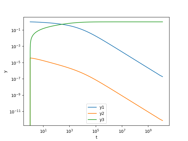
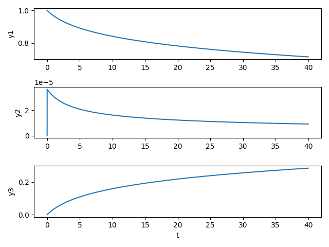
SciPyのodeintを用いて以下のOrdinary Differential Equations (ODE)を解き，文献[1,2]のRobertson problemの数値解を再現する．

$\displaystyle y_1^{\prime} = -0.04 y_1 + 10^4 y_2 y_3$

$\displaystyle y_2^{\prime} = 0.04 y_1 - 10^4 y_2 y_3 - 3 \times 10^7 y_2^2$

$\displaystyle y_3^{\prime} = 3 \times 10^7 y_2^2$

ここで，初期値 $y_1 \left( 0 \right) = 1.0$ ， $y_2 \left( 0 \right) = 0.0$ ， $y_3 \left( 0 \right) = 0.0$ である．

[1] Thohura, S. and Rahman, A., Numerical Approach for Solving Stiff Differential Equations: A Comparative Study, GLOBAL JOURNAl OF SCIENCE FRONTIER RESEARCH MATHEMATICS AND DECISION SCIENCES, 13 (6) (2013)

[2] The Robertson Problem — Dymos

#
# Robertson problem in
# Thohura, S. and Rahman, A.,
# Numerical Approach for Solving Stiff Differential Equations:
# A Comparative Study,
# GLOBAL JOURNAl OF SCIENCE FRONTIER RESEARCH
# MATHEMATICS AND DECISION SCIENCES, 13 (6) (2013)
#
import numpy as np
from scipy.integrate import odeint
import matplotlib.pyplot as plt

# right-hand side
def rhs(y, x):
    k1 = 0.04
    k2 = 3e7
    k3 = 1e4
    return [-k1*y[0] + k3*y[1]*y[2],
             k1*y[0] - k3*y[1]*y[2] - k2*y[1]**2,
                                      k2*y[1]**2]

# initial condition
y0 = [1.0, 0.0, 0.0]

# output interval
p = np.arange(0.0, 10.1, 0.001)
x = np.empty(10100)
i = 0
for t in p:
    x[i] = 10.0**t
    i += 1

# solve ode
y = odeint(rhs, y0, x)

# output
plt.xlabel('t')
plt.ylabel('y')
plt.xscale('log')
plt.yscale('log')
plt.plot(x, y[:,0], label='y1')
plt.plot(x, y[:,1], label='y2')
#plt.plot(x, y[:,1]*1e4)
plt.plot(x, y[:,2], label='y3')
plt.legend()
#plt.show()
plt.savefig('Thohura2013-Fig1.png')